When you see body-in-white samples doing repetitive cycles for an R&R study of the robot programming, you are starting to get close.
Then pathfinder units need to be evaluated and tested before making a thousand mistakes before you catch it.
Here's what the most modern mfr'g does. Using statistical control analysis, they run enough operations to determine CpK values. This is Process Capability. How often does it screw up? All processes have a failure rate, so you aim for a target, ideally 6 sigma.
We can look at 120 components and tell how many faulty ones will exist in a lot of 1,000,000. But you also need to keep testing sample batches during production to determine the decay or anomalies of the CpK levels.
Production can start before you have 6-sigma confidence, you still do the same acceptance tests, and the line not up to 6-sigma just means your rework rate is higher than you want.
Just to get a feel, at 6-sigmal, each process has a fail rate of 2 parts in a billion, if you have 100 steps in the assembly, then your chance of getting a good end-product without rework is 0.999999998^100, or fail rate (bad car) of 0.2 in 1 million. If you have 1,000 steps, then fail rate goes up to 2 bad cars in 1 million, and 10,000 steps gives you chance of 20 bad cars in 1 million. So 6-sigma is very very strict, failure rate is very close to 0.
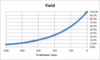
For early production for sure you won't hit this rate. For example out of 10,000 steps, 1,000 of them are not yet well controlled, and your variability on them is 2x as large as you wanted, so you get 3 sigma, which gives a fail rate of 0.27% per step. Aggregating these 1,000 steps, your yield of getting a good car is 0.9973^1000=6.7%, so almost certainly you will need to rework. If you can fix most of them, and only have 100 problematic steps left, then your yield is 0.9973^100=76.3%, now you're doing a lot better. If you plot the yield vs # of problematic steps using the above example, you get this:
However the last few problems are usually the hardest to fix so they would take longer in terms of time, so if you translate this trend to have time on x-axis, the last few problems (to the right side of the plot) will have their x-axis stretched out, so you end with the "S" curve